Polynomial Regression comparison on Advertising data

Problem Statement: We analyzed simple linear regression in our last article and compared TV and newspaper spend and if we can draw a correlation with sales. In this article, we will do same comparison but using polynomial fit. We will be fitting higher degree polynomial ,say, third order equation.

Data is downloaded from Kaggle

Polynomial fit equation third degree

y = B3*X**3 + B2*X**2 + B1*X + B0

which is B3 (coefficient) times X to the power 3 + B2 times X to the power 2+ B1 times X + B0

We will use our same np.polyfit, but before lets do the essentials and import all the libraries and read our csv

Import your Libraries

import numpy as np
import pandas as pd
import matplotlib.pyplot as plt
import seaborn as sns

Load the file

file_path = r'/Users/Downloads/advertising.csv'
df_ad_data = pd.read_csv(file_path)
df_ad_data.head()

X_TV = df_ad_data['TV']
y_tv = df_ad_data['Sales']

TV

Polynomial Regression

beta_tv_3, beta_tv_2, beta_tv_1, beta_tv_0 = np.polyfit(X_TV, y_tv, deg = 3)

As you can see above the value of degree is third order which will give us 4 coefficients. These coefficient is what we will use in our polynomial equation y = B3*X**3 + B2*X**2 + B1*X + B0 to substitute B3, B3, B1 and B0.

Now, we can generate some potential spend for TV for which we can get some predicted sales value

potential_tv_spend_poly = np.linspace(0, 300, 100)

predicted_tv_sales_poly = (beta_tv_3*potential_tv_spend_poly**3)+(beta_tv_2*potential_tv_spend_poly**2)+(beta_tv_1*potential_tv_spend_poly)+beta_tv_0

And now the plotting begins

sns.scatterplot(data=df_ad_data, x='TV', y='Sales')
plt.plot(potential_tv_spend_poly, predicted_tv_sales_poly, color='red')

If we compare the results of this polynomial fit with the linear fit in previous article, it is difficult to evaluate visually and say one is better fit than other. In order to better evaluate we will have to start calculating error on each fit. In our future articles we will start doing this so as to give us a better understanding into model performance.

Newspaper

We will use polynomial regression to see how it compares with linear fit for newspaper in previous article.

First, lets get our series ready

X_Newspaper = df_ad_data['Newspaper']
y_newspaper = df_ad_data['Sales']

Calculating coefficients for Polynomial Regression

beta_np_3, beta_np_2, beta_np_1, beta_np_0 = np.polyfit(X_Newspaper, y_newspaper, deg = 3)

Calculating potential spend for newspaper

potential_newspaper_spend = np.linspace(0,100, 100)

Calculating predicted spend for Newspaper

predicted_newspaper_sales_poly = (beta_np_3*potential_newspaper_spend**3)+(beta_np_2*potential_newspaper_spend**2)+(beta_np_1*potential_newspaper_spend)+beta_np_0

Let’s plot it now

sns.scatterplot(data=df_ad_data, x='Newspaper', y='Sales')
plt.plot(potential_newspaper_spend, predicted_newspaper_sales_poly, color='r')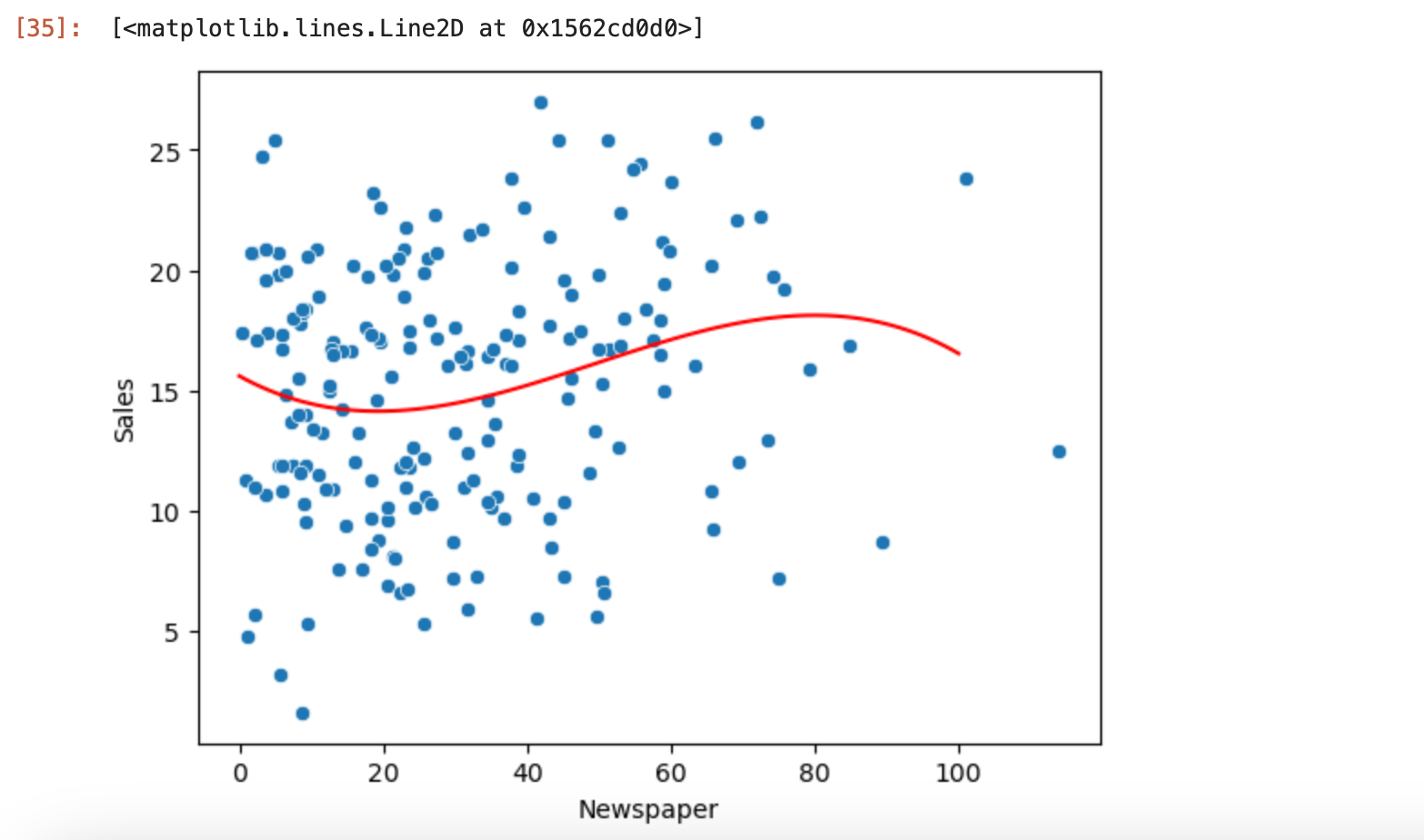

For newspaper we can make a quick determination that even a polynomial fit is not ideal. However, as stated above we have a motivation to calculate the error to see which algorithm would be better suitable.

More to come, stay tuned for next article.

With that we have reached the end of this article. Thank you once again for reading.